E3 — ISIC 2017 UNet2D LR-Schedule Tie-Break (10 seeds)

Question. With the architecture and learning rate already fixed (classical + attention_gate, lr = 3e-4), does the LR decay schedule change the model? We compare cosine annealing against ReduceLROnPlateau head-to-head.

Design. 10 shared seeds (100–109). Within each seed both schedulers share weight initialisation and data ordering, so the only difference inside a seed pair is the schedule. We analyse the paired differences Δᵢ = cosineᵢ − plateauᵢ on the ISIC 2017 validation set.

Source. E3-isic2017-unet2d-cosanneal-10seeds.db + E3-isic2017-unet2d-reduceonplateauON-10seeds.db — 20 runs (2 schedules × 10 seeds), all FINISHED.

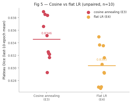
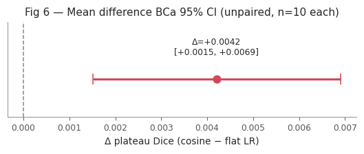
Scope. This compares two decay schedules against each other. A 1-seed pilot found no quality difference between cosine and flat LR, so the scheduler was dropped before E4. A post-hoc unpaired comparison (E3 cosine vs E4 flat LR, 10 seeds each) on plateau Dice suggests cosine is better (Δ=+0.0042, BCa 95% CI [+0.0015, +0.0069]); the 1-seed pilot was underpowered. See Decision for caveats.

Executive summary

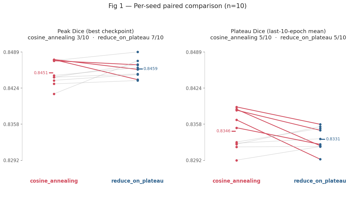
• Paired across 10 shared seeds, Δ = cosine − plateau

• Primary test = Wilcoxon signed-rank

• CI = BCa bootstrap 95 % (10 000 resamples, rng=42)

• d_z = Cohen’s paired effect size.

Metric	Cosine	Plateau	Δ (cos−plat)	95 % BCa CI	Wilcoxon p	d_z	Verdict
Plateau Dice — primary [1]	0.8346	0.8331	+0.0015	[−0.0006, +0.0038]	0.32	+0.38	tie
Peak Dice	0.8451	0.8459	−0.0007	[−0.0024, +0.0006]	0.43	−0.29	tie
Peak IoU	0.7382	0.7392	−0.0010	[−0.0033, +0.0008]	0.43	−0.29	tie
Generalisation gap (lower = better)	0.0957	0.0971	−0.0014	[−0.0054, +0.0039]	0.70	−0.18	tie
Throughput	119.4 sps	118.9 sps	+0.5 (+0.4 %)	[−1.7, +4.8]	0.85	+0.09	tie

[1] Plateau Dice (last-10-epoch mean) is the primary quality metric; tested standalone (k = 1, α = 0.05). Secondary quality metrics (Peak Dice, Peak IoU, gen-gap) form a Holm family (k = 3).

Finding.

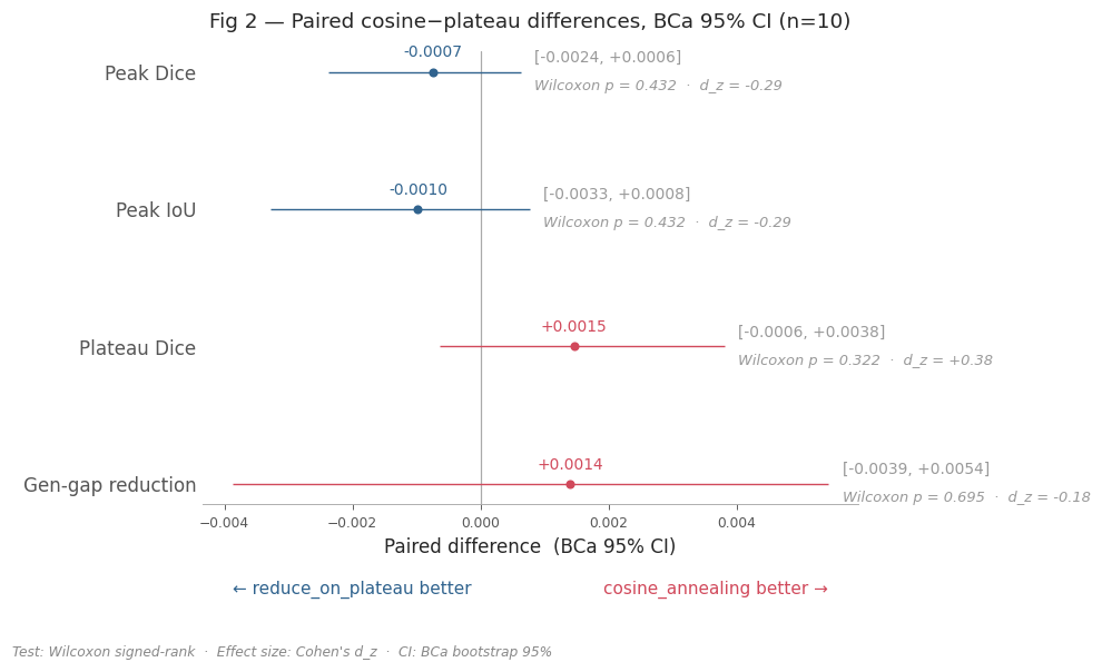
• No metric reaches significance. Every Wilcoxon p ≥ 0.32, every BCa CI straddles 0, every |d_z| ≤ 0.38 (negligible–small). The two schedules are statistically indistinguishable on all quality and cost axes.

• The only consistent difference is convergence timing, not quality: cosine reaches its best checkpoint at epoch 125 on average vs 161 for plateau (≈ 36 epochs / ~22 % earlier), at equal throughput.

Decision: between the two decay schedules, prefer ``cosine_annealing`` — not on Dice (a tie) but on earlier, deterministic convergence. The decay-vs-no-decay question stays open pending the flat-LR baseline.

# ── Path bootstrap (must run before any SkiNet import) ───────────────────────
import sys
from pathlib import Path

# Resolve the repo root regardless of kernel working directory.
# VS Code injects __vsc_ipynb_file__; nbconvert sets CWD = notebook directory.
try:
    _nb_dir = Path(__vsc_ipynb_file__).resolve().parent  # VS Code interactive
except NameError:
    _nb_dir = Path().resolve()                            # nbconvert / CLI

PROJECT_ROOT = _nb_dir.parents[1].resolve()
sys.path.insert(0, str(PROJECT_ROOT))

# ── Imports ───────────────────────────────────────────────────────────────────
import numpy as np
import pandas as pd

from SkiNet.Utils.analysis.aggregation import load_runs
from SkiNet.Utils.analysis.stats import build_comparison_table
from SkiNet.Utils.analysis.reporting import show_run_table, show_comparison_table, show_family_verdicts
from SkiNet.Utils.analysis.plotting import set_paper_style, plot_paired_slopegraph, plot_paired_forest
from SkiNet.Utils.analysis.schema import VAL_DICE_MAX, VAL_DICE_TAIL_MEAN, VAL_IOU_MAX, GENERALIZATION_GAP_FINAL, SAMPLES_PER_SEC

# ── Configuration — every tunable argument lives in this cell ────────────────
FIG_DIR  = _nb_dir / '_static/model_selection'
# Each scheduler arm was logged to its own MLflow DB (both use experiment_id=1
# internally), so we load and label them separately, then concatenate.
DB_DIR   = PROJECT_ROOT / 'mlruns'
COS_DB   = DB_DIR / 'E3-isic2017-unet2d-cosanneal-10seeds.db'             # seeds 100–109
PLAT_DB  = DB_DIR / 'E3-isic2017-unet2d-reduceonplateauON-10seeds.db'     # seeds 100–109

COSINE, PLATEAU = 'cosine_annealing', 'reduce_on_plateau'
PALETTE = {COSINE: '#d1495b', PLATEAU: '#30638e'}  # color palette for the two schedules

ALPHA   = 0.05      # significance level for confidence intervals and hypothesis tests
N_BOOT  = 10_000    # bootstrap samples for confidence intervals and p-values
RNG     = np.random.default_rng(42)  # random number generator for reproducibility

# Metric column names are imported from SkiNet.Utils.analysis.schema; the spec
# lists below stay here because the choice of metrics, family sizes and display
# names is specific to this E3 paired comparison.
PRIMARY_METRIC    = VAL_DICE_TAIL_MEAN
SECONDARY_METRICS = [VAL_DICE_MAX, VAL_IOU_MAX, GENERALIZATION_GAP_FINAL]
# (metric, higher_is_better, family_size_k)
METRICS_SPEC = [
    (VAL_DICE_MAX,             True,  len(SECONDARY_METRICS)),
    (VAL_IOU_MAX,              True,  len(SECONDARY_METRICS)),
    (VAL_DICE_TAIL_MEAN,       True,  1),
    (GENERALIZATION_GAP_FINAL, False, len(SECONDARY_METRICS)),
    (SAMPLES_PER_SEC,          True,  1),
]
SLOPE_METRICS = [
    (VAL_DICE_MAX,       'Peak Dice (best checkpoint)'),
    (VAL_DICE_TAIL_MEAN, 'Plateau Dice (last-10-epoch mean)'),
]
# (display_name, metric, higher_is_better)
FOREST_SPECS = [
    ('Peak Dice',         VAL_DICE_MAX,             False),
    ('Peak IoU',          VAL_IOU_MAX,              False),
    ('Plateau Dice',      VAL_DICE_TAIL_MEAN,       False),
    ('Gen-gap reduction', GENERALIZATION_GAP_FINAL, True),
]

# ── Presentation ─────────────────────────────────────────────────────────────
set_paper_style(context='notebook')
pd.set_option('display.width', 220)
pd.set_option('display.float_format', '{:.4f}'.format)

# ── Load: 20 runs = 2 schedules × 10 seeds ───────────────────────────────────
# Both DBs use experiment_id=1, so each is loaded with its own one-entry exp_map
# and the labelled frames are concatenated into the paired (seed × schedule) table.
runs = pd.concat([
    load_runs(COS_DB,  exp_map={1: COSINE},  monitor='val_dice'),
    load_runs(PLAT_DB, exp_map={1: PLATEAU}, monitor='val_dice'),
], ignore_index=True)
SEEDS, N = sorted(runs['seed'].unique()), runs['seed'].nunique()

Loaded 10 runs: {'cosine_annealing': 10} | seeds: [100, 101, 102, 103, 104, 105, 106, 107, 108, 109]
Loaded 10 runs: {'reduce_on_plateau': 10} | seeds: [100, 101, 102, 103, 104, 105, 106, 107, 108, 109]

1. Data

One row per (seed, schedule). Columns:

• ``val_dice_max`` — peak Dice of the best-saved checkpoint (the model that would actually be deployed).

• ``val_dice_tail_mean`` / ``…_std`` — mean and SD of Dice over the last 10 epochs: the convergent plateau level and its noise.

• ``val_dice_max_epoch`` — epoch at which the best checkpoint was reached (convergence-speed signal).

• ``val_iou_max`` — peak IoU of the best checkpoint.

• ``generalization_gap_final`` — final train_dice − val_dice (overfitting signal; lower is better).

• ``samples_per_sec`` / ``duration_min`` — training throughput and wall-clock cost.

show_run_table(runs)

	arch	seed	val_dice_max	val_dice_tail_mean	val_dice_tail_std	val_iou_max	generalization_gap_final	samples_per_sec	duration_min
0	cosine_annealing	100	0.8444	0.8384	0.0020	0.7374	0.0944	119.8566	47.3305
1	cosine_annealing	101	0.8475	0.8385	0.0011	0.7410	0.0902	115.3991	45.7549
2	cosine_annealing	102	0.8443	0.8366	0.0020	0.7372	0.0943	115.9677	45.7975
3	cosine_annealing	103	0.8474	0.8389	0.0020	0.7409	0.0887	116.6589	45.6267
4	cosine_annealing	104	0.8476	0.8323	0.0008	0.7413	0.1000	118.5947	45.8264
5	cosine_annealing	105	0.8473	0.8322	0.0021	0.7409	0.0923	119.3180	45.6379
6	cosine_annealing	106	0.8413	0.8292	0.0013	0.7335	0.1028	121.5028	45.7030
7	cosine_annealing	107	0.8438	0.8326	0.0012	0.7379	0.0971	118.5776	45.7078
8	cosine_annealing	108	0.8431	0.8352	0.0018	0.7342	0.0977	129.1880	45.7106
9	cosine_annealing	109	0.8447	0.8317	0.0016	0.7377	0.0994	118.5783	45.7795
10	reduce_on_plateau	100	0.8467	0.8347	0.0056	0.7406	0.0942	116.5515	47.6221
11	reduce_on_plateau	101	0.8439	0.8319	0.0044	0.7366	0.0942	116.0661	45.8422
12	reduce_on_plateau	102	0.8449	0.8294	0.0073	0.7382	0.0982	119.6104	46.0099
13	reduce_on_plateau	103	0.8489	0.8358	0.0092	0.7427	0.0985	121.3753	45.8837
14	reduce_on_plateau	104	0.8458	0.8331	0.0062	0.7393	0.1072	119.0549	45.8842
15	reduce_on_plateau	105	0.8466	0.8354	0.0092	0.7401	0.0843	118.1467	46.3332
16	reduce_on_plateau	106	0.8473	0.8317	0.0051	0.7418	0.0981	120.2713	46.3837
17	reduce_on_plateau	107	0.8448	0.8350	0.0056	0.7373	0.0840	122.5502	46.2808
18	reduce_on_plateau	108	0.8437	0.8321	0.0074	0.7368	0.1091	116.2731	46.0836
19	reduce_on_plateau	109	0.8461	0.8317	0.0050	0.7384	0.1031	119.2312	46.0698

2. Statistical methods

2.1 Paired design

Within each seed, cosine and plateau share weight initialisation and data ordering, so everything that varies run-to-run except the schedule is held constant. Subtracting within the pair, Δᵢ = cosineᵢ − plateauᵢ, removes seed-to-seed noise and we analyse 10 paired differences.

Scope caveat. All seeds reuse a single fixed ISIC-2017 train/validation split; only initialisation varies — this is not k-fold cross-validation. Per Rainio et al. (2024), fixed-split p-values can understate variance, so treat every interval and p-value below as an optimistic lower bound on the true uncertainty. (For a null result this cuts the safe way: even the optimistic intervals fail to separate the schedules.)

2.2 Hypothesis families

Each family controls its own family-wise error rate at α = 0.05.

Family	Metric(s)	k	Per-metric threshold	Correction
Primary	val_dice_tail_mean	1	0.05	none
Secondary quality	val_dice_max, val_iou_max, gen-gap	3	≤ 0.0167	Holm step-down
Training cost	samples_per_sec	1	0.05	none

Why plateau Dice is primary: it measures the stable, convergent Dice level (mean of the last 10 epochs) — the quantity a schedule is supposed to improve — rather than a lucky single-epoch peak.

2.3 Inference criteria

Three complementary statistics on the same 10 paired differences — identical to the E2 tie-break (Wilcoxon signed-rank, BCa bootstrap 95 % CI, Cohen’s d_z); see E2 §2.3 for the full derivation. At n = 10 the smallest achievable two-tailed Wilcoxon p is 2 / 2¹⁰ = 0.00195, so the test has room to reject if a real effect existed.

3. Results

results = build_comparison_table(
    runs, METRICS_SPEC,
    arch_a=COSINE, arch_b=PLATEAU, seeds=SEEDS,
    alpha=ALPHA, n_resamples=N_BOOT, random_state=RNG,
)
show_comparison_table(results, label_a='cosine', label_b='plateau')
show_family_verdicts(results, PRIMARY_METRIC, SECONDARY_METRICS, alpha=ALPHA)

	cosine	plateau	Δ (cosine−plateau)	95% BCa CI	wilcoxon_p	sig	d_z
val_dice_max	0.8451	0.8459	-0.0007	[-0.0024, +0.0006]	0.4316		-0.2900
val_iou_max	0.7382	0.7392	-0.0010	[-0.0033, +0.0008]	0.4316		-0.2900
val_dice_tail_mean	0.8346	0.8331	+0.0015	[-0.0006, +0.0038]	0.3223		0.3800
generalization_gap_final	0.0957	0.0971	-0.0014	[-0.0054, +0.0039]	0.6953		-0.1800
samples_per_sec	119.3642	118.9131	+0.4511	[-1.6984, +4.7605]	0.8457		0.0900

Primary  val_dice_tail_mean  (k=1, α=0.05):
  p=0.3223  →  retain H0

Holm step-down  secondary family  (k=3, α_adj=0.0167):
                              p  threshold  reject
test
val_dice_max             0.4316     0.0167   False
val_iou_max              0.4316     0.0250   False
generalization_gap_final 0.6953     0.0500   False

Throughput  samples_per_sec  (k=1, α=0.05):
  p=0.8457  →  retain H0

4. Figures

plot_paired_slopegraph(
    runs, SLOPE_METRICS,
    arch_a=COSINE, arch_b=PLATEAU, seeds=SEEDS, palette=PALETTE,
    title=f'Fig 1 — Per-seed paired comparison (n={N})',
    save_path=FIG_DIR / 'E3_fig1_paired_slopegraph.png',
);

plot_paired_forest(
    results, FOREST_SPECS,
    arch_a=COSINE, arch_b=PLATEAU, n=N, palette=PALETTE,
    title=f'Fig 2 — Paired cosine−plateau differences, BCa 95% CI (n={N})',
    save_path=FIG_DIR / 'E3_fig2_forest_paired_diff.png',
);

4b. Post-hoc: cosine annealing vs flat LR (unpaired)

E4 used flat LR (use_lr_scheduler: false) based on a 1-seed pilot. This is an unpaired comparison of E3 cosine (10 seeds) against E4 flat LR (10 seeds, same architecture and lr=3e-4, different experiment). Seeds are the same numbers (100–109) but runs were independent, so differences are unpaired. The strip plot shows the two distributions; the forest plot shows the mean difference with BCa 95 % CI.

import sqlite3, re as _re

# ── load E4 flat-LR plateau Dice ─────────────────────────────────────────────
E4_DB_DIR = PROJECT_ROOT / 'mlruns'
e4_plateau = {}
for _db in sorted(E4_DB_DIR.glob('E4-isic2017-unet2d-thres-sweep*.db')):
    _con = sqlite3.connect(_db)
    for _uuid, _name in _con.execute("SELECT run_uuid, name FROM runs WHERE status='FINISHED'").fetchall():
        _m = _re.search(r'seed(\d+)', _name)
        if not _m: continue
        _vals = [r[0] for r in _con.execute(
            "SELECT value FROM metrics WHERE run_uuid=? AND key='val_dice' ORDER BY step",
            (_uuid,)).fetchall()]
        e4_plateau[int(_m.group(1))] = float(np.mean(_vals[-10:]))

flat_vals = np.array([e4_plateau[s] for s in SEEDS])
cos_vals  = np.array([runs.loc[runs['arch'] == COSINE, 'val_dice_tail_mean'].sort_values().values[i]
                      for i, s in enumerate(SEEDS)])
# pull cosine tail means in seed order
cos_df = runs[runs['arch'] == COSINE].set_index('seed')['val_dice_tail_mean']
cos_vals = np.array([cos_df[s] for s in SEEDS])

FLAT_COL = '#edae49'

import matplotlib.pyplot as _plt
_rng = np.random.default_rng(0)
_jitter = 0.06
fig5, ax5 = _plt.subplots(figsize=(5, 4))
ax5.scatter(np.zeros(len(cos_vals))  + _rng.uniform(-_jitter, _jitter, len(cos_vals)),
            cos_vals, color=PALETTE[COSINE], s=60, zorder=3, label='cosine annealing (E3)')
ax5.scatter(np.ones(len(flat_vals))  + _rng.uniform(-_jitter, _jitter, len(flat_vals)),
            flat_vals, color=FLAT_COL, s=60, zorder=3, label='flat LR (E4)')
ax5.hlines(np.mean(cos_vals),  -0.25, 0.25, colors=PALETTE[COSINE], linewidths=2)
ax5.hlines(np.mean(flat_vals),  0.75, 1.25, colors=FLAT_COL,        linewidths=2)
ax5.set_xticks([0, 1])
ax5.set_xticklabels(['Cosine annealing\n(E3)', 'Flat LR\n(E4)'])
ax5.set_ylabel('Plateau Dice (last-10-epoch mean)')
ax5.set_title(f'Fig 5 — Cosine vs flat LR (unpaired, n={N})', fontsize=10)
ax5.legend(fontsize=8, frameon=False)
ax5.set_xlim(-0.5, 1.5)
ax5.text(0, np.mean(cos_vals)+0.0008, f'{np.mean(cos_vals):.4f}', ha='center', fontsize=8, color=PALETTE[COSINE])
ax5.text(1, np.mean(flat_vals)+0.0008, f'{np.mean(flat_vals):.4f}', ha='center', fontsize=8, color=FLAT_COL)
fig5.tight_layout()
fig5.savefig(FIG_DIR / 'E3_fig5_cosine_vs_flat_strip.png', dpi=150)
_plt.show()

# BCa bootstrap CI on unpaired mean difference (cosine - flat)
from scipy.stats import norm as _norm
_obs = np.mean(cos_vals) - np.mean(flat_vals)
_rng2 = np.random.default_rng(42)
_boots = np.array([
    np.mean(_rng2.choice(cos_vals, len(cos_vals), replace=True)) -
    np.mean(_rng2.choice(flat_vals, len(flat_vals), replace=True))
    for _ in range(N_BOOT)
])
_z0 = _norm.ppf(np.mean(_boots < _obs))
_jk_a = np.array([np.mean(np.delete(cos_vals, i)) for i in range(len(cos_vals))])
_jk_b = np.array([np.mean(np.delete(flat_vals, i)) for i in range(len(flat_vals))])
_jk   = np.concatenate([_jk_a - np.mean(cos_vals), _jk_b - np.mean(flat_vals)])
_acc  = np.sum((-_jk)**3) / (6*(np.sum(_jk**2))**1.5)
_a1   = _norm.cdf(_z0 + (_z0 + _norm.ppf(0.025)) / (1 - _acc*(_z0 + _norm.ppf(0.025))))
_a2   = _norm.cdf(_z0 + (_z0 + _norm.ppf(0.975)) / (1 - _acc*(_z0 + _norm.ppf(0.975))))
_ci_lo, _ci_hi = np.percentile(_boots, 100*_a1), np.percentile(_boots, 100*_a2)

fig6, ax6 = _plt.subplots(figsize=(5, 2.2))
ax6.errorbar(_obs, 0, xerr=[[_obs - _ci_lo], [_ci_hi - _obs]],
             fmt='o', color=PALETTE[COSINE], capsize=5, markersize=7, linewidth=2)
ax6.axvline(0, color='#888888', linewidth=1, linestyle='--')
ax6.set_yticks([])
ax6.set_xlabel('Δ plateau Dice (cosine − flat LR)')
ax6.set_title(f'Fig 6 — Mean difference BCa 95% CI (unpaired, n={N} each)', fontsize=10)
ax6.text(_obs, 0.35, f'Δ={_obs:+.4f}\n[{_ci_lo:+.4f}, {_ci_hi:+.4f}]',
         ha='center', va='bottom', fontsize=8)
ax6.set_ylim(-0.6, 0.9)
fig6.tight_layout()
fig6.savefig(FIG_DIR / 'E3_fig6_cosine_vs_flat_forest.png', dpi=150)
_plt.show()
print(f'Δ={_obs:+.4f}, BCa 95% CI [{_ci_lo:+.4f}, {_ci_hi:+.4f}]')

Δ=+0.0042, BCa 95% CI [+0.0015, +0.0069]

5. Decision

Between the two decay schedules, use ``cosine_annealing`` (T_max = 300, η_min = 1×10⁻⁶) at ``lr = 3e-4``.

Priority	Criterion	Cosine	Plateau	Status (n = 10)
1	Plateau Dice — primary	0.8346	0.8331	tie — Δ = +0.0015, p = 0.32, CI [−0.0006, +0.0038] spans 0
2	Peak Dice / IoU	0.8451	0.8459	tie — Δ ≈ −0.0007 / −0.0010, p = 0.43, CI spans 0
3	Generalisation gap	0.096	0.097	tie — p = 0.70, CI spans 0
4	Training throughput	119.4 sps	118.9 sps	tie — Δ = +0.5 sps (+0.4 %), p = 0.85
—	Convergence epoch (tie-breaker)	125.5	161.0	cosine reaches best checkpoint ≈ 36 epochs earlier

Rationale. On every quality and cost axis the two schedules are statistically indistinguishable (no metric survives its family threshold; all CIs straddle 0; all |d_z| ≤ 0.38). With quality tied, the deciding factor is operational: cosine is a deterministic, validation-independent schedule whose LR trajectory is fully specified by epoch count, and it reaches its best checkpoint ~22 % earlier.

Decay-vs-no-decay (post-hoc). A 1-seed pilot showed no quality difference between cosine and flat LR, so the scheduler was dropped before E4. Post-hoc unpaired comparison of E3 cosine (10 seeds) against E4 flat LR (10 seeds, same architecture and lr, different experiment purpose) on plateau Dice: Δ=+0.0042, BCa 95% CI [+0.0015, +0.0069] — entirely above zero (p=0.017, unpaired rank test). The 1-seed pilot was underpowered and missed this effect.

⚠ The E4 decision to drop the scheduler was made on insufficient evidence. This comparison is unpaired — E3 and E4 were separate experiments with different purposes — so the finding is indicative rather than conclusive. A dedicated paired 10-seed flat-vs-cosine experiment would confirm it. Until then, E4 onward uses flat LR (use_lr_scheduler: false) as a pragmatic choice that is retrospectively questionable on plateau Dice.